Physics Informed Neural Networks and JAX
This is a short blog plost explaining the idea behind physics informed neural networks (PINNs) and how to implement one using JAX, a high-performance machine learning library.
This example is heavily inspired by Ben Moseley’s post on PINNs. I use the same example of the damped harmonic oscillator but implement it in JAX instead of PyTorch.
The physics
The problem we would like to solve is that of the damped harmonic oscillator in one dimension, which you can think of as a spring oscillating with ever decreasing amplitude due to friction. This system can be described by the following differential equation:
\[m\frac{d^2x}{dt^2} + c\frac{dx}{dt} + kx = 0\]Here, \(x\) is the deviation from the equillibrium point (point of rest), \(m\) is the mass of the oscillating object and \(c\) and \(k\) are constants declaring the strength of friction and of the force pulling the object back towards \(x = 0\).
The solution to this differential equation (DE) would be an equation \(x(t)\) which satisfies the upper equation and tells us the position \(x\) of the object at timestep \(t\), given some initial conditions. The equation \(x(t)\) is exactly what our network will learn and we will use the DE as an additional loss term to help the network learn the underlying physics of the problem.
Generating the training data
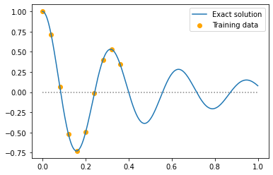
We will use the analytical solution of the damped harmonic oscillator to generate training data for the network. In a more elaborate example these points would come from a physical simulator, e.g. a finite difference method.
Using the solution, we create a graph \(x(t)\) of the oscillator given some initial conditions and sample 10 points (orange dots) to use a training data for the network.
The network and a physics-agnostic loss
We will use a three layer MLP with 32 neurons per layer and Tanh activation functions. The network has one input \(t\) and one output \(x\). By itself, JAX does not have many tools for implementing neural networks and training them but there are multiple ML libraries built on top of it to do just that. Here we’ll use Haiku for building the network and Optax for training it. Both libraries are open-source and maintained by DeepMind.
Below is the code for defining the MLP using Haiku, calculating the MSE loss between the network’s
prediction and the training data and finally running one update step. We use jax.grad to calculate
the gradient of the loss with respect to the model parameters.
jax.grad is one of multiple function transformations JAX provides which takes a scalar-valued
function as input and calculates the gradient of the output of this function (here: the MSE loss)
with respect to its first input (here: the network’s params). The optimizer, we’ll use Adam, then
takes these gradients, calculates the parameter updates and finally applies them.
# Create three layer MLP
def net_fn(t: jnp.ndarray) -> jnp.ndarray:
    mlp = hk.Sequential([
        hk.Linear(32), jax.nn.tanh,
        hk.Linear(32), jax.nn.tanh,
        hk.Linear(32), jax.nn.tanh,
        hk.Linear(1)
    ])
    return mlp(t)

# Calculate mean squared error loss
def loss(params: hk.Params, t: jnp.ndarray, x: jnp.ndarray) -> jnp.ndarray:
    x_pred = net.apply(params, t)
    mse = jnp.mean((x_pred - x)**2)
    return mse

@jax.jit
def update(params: hk.Params, opt_state: optax.OptState, t: jnp.array, x: jnp.array):
    grads = jax.grad(loss)(params, t, x)
    updates, opt_state = opt.update(grads, opt_state)
    new_params = optax.apply_updates(params, updates)
    return new_params, opt_state
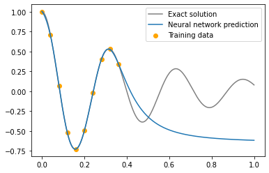
If we now train this network on the 10 data points we sampled earlier, we can see that it fits the training data pretty well but quickly diverges after that. This is not very surprising, as the loss only includes the distance to the training data and provides no further information outside of that. So far the model has no knowledge of the physical system generating the data and this is where the differential equation we described earlier comes into the picture.
A physics-informed loss
Let’s first recap what our loss function looks like so far and then show how we can extend it to include the differential equation.
\[L_{data} = \frac{1}{N} \sum_{i}^N (x_{NN}(t_i; \theta) - x_{true}(t_i))^2\]This naive loss only minimizes the distance between the training data and the network’s prediction at some sampled timesteps \(t\). When we remember that the model, parameterised by weights \(\theta\), is supposed to learn the function \(x(t)\), we can include an additional piece of information in the loss function. Namely, that the derivatives \(\frac{dx}{dt}\) and \(\frac{d^2x}{dt^2}\) should satisfy the differential equation we introduced earlier:
\[m\frac{d^2x}{dt^2} + c\frac{dx}{dt} + kx = 0\]Leading to the following physics-informed loss:
\[L = L_{data} + \lambda L_{DE}\] \[L_{DE} = \frac{1}{M} \sum_{j}^M ([m \frac{d^2}{dt^2} + c \frac{d}{dx} + k] x_{NN}(t_j; \theta) )^2\]Where \(L_{DE}\) makes sure that the network and its first and second order derivatives match the differential equation at different inputs \(t_j\). Using this kind of loss is the idea behind Physics-Informed Neural Networks [1] (PINNs for short).
To calculate the \(L_{DE}\) loss we need to calculate the first and second order derivative of the
neural network \(x(t; \theta)\) with respect to its input \(t\). Thanks to Jax’s jax.grad
doing this is fairly straightforward, as can be seen in the code sample below.
def loss_physics(params: hk.Params, t_data: jnp.array, x_data: jnp.array, t_physics: jnp.array):
    x_pred_data = net.apply(params, t_data)
    data_loss = jnp.mean((x_pred_data - x_data)**2)

    # The solution to the differential equation is represented by our network
    x = lambda t: net.apply(params, t)[0]

    # Calculate first and second derivates of network (x) with respect to input (t)
    # Remember: The network is the solution to the differential equation
    x_dt = jax.vmap(jax.grad(x))
    x_dt2 = jax.vmap(jax.grad(lambda t: jax.grad(x)(t)[0]))

    # Compute physical loss
    y_pred_physics = net.apply(params, t_physics)
    residual = x_dt2(t_physics) + mu * x_dt(t_physics) + k * x_pred_physics
    physics_loss = (1e-4) * jnp.mean(residual**2)

    return data_loss + physics_loss
The important lines here are the three where we define the x, x_dt and x_dt2 functions.
net.apply(params, t) feeds the \(t\) value through the network and returns an output tensor of shape
(1,). Because jax.grad only works on scalar-valued functions we have to index into the array and
return the single element. To make this easy we define a lambda function x(t) which takes a \(t\) as
input and returns the corresponding \(x(t)\), predicted by the network. Using this function, we can
now easily calculate the first derivative \(\frac{dx}{dt}\) by applying jax.grad to x.
Because we would like to evaluate x_dt on batches of shape (M, 1) instead of just individual
values, we apply jax.vmap to the function returned by jax.grad(x). vmap(f)
is another one of JAX’s function transformations and adds an additional batch axis to the input and
output of a function f, thus automatically turning the dimension of jax.grad(x) from (1) -> (1)
into (M, 1) -> (M, 1). We then use jax.grad twice to obtain the second derivative x_dt2,
again indexing into the returned tensor to obtain a scalar value and using jax.vmap to
automatically add a batch dimension. The [0] index in the two lambda functions might seem a bit
weird here but it would be absolutely necessary if we had a network (physical model) with multiple
inputs or outputs.
After this we use x, x_dt and x_dt2 to calculate the physics loss \(L_{DE}\) (“residual”) and
add it to the data loss \(L_{data}\) with a scaling factor \(\lambda = 10^{-4}\).
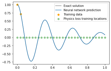
The trained network now matches the theoretical model over the whole time range and only requires two data points to converge to the correct solution. The plot below shows the solution after 20k training steps and the green dots represent the time points \(t_j\) where we evaluated the first and second order derivative.
I personally think that using JAX to write this code is an amazing experience. Calculating the first and
second order derivative of any function is fairly straightforward thanks to jax.grad and
creating a batched version of a calculation is as easy as calling jax.vmap on it.
There are many more great function transformations JAX has to offer, like jax.pmap
or jax.jit
and the official documentation contains fairly comprehensive
tutorials and explanations. Overall, using JAX makes your code look very similar to the underlying
equations and while there are some subtleties to using it (most of them due to the fact that JAX’s function
transformations work on pure functions), the sharp bits can be fairly easily avoided or abstracted
away by using libraries like Haiku.
Conclusion
We saw how adding a physics-informed loss in the form of a differential equation can help the model generalize and make correct predictions far away from the training data. While we looked at a fairly simply problem here, physics-informed neural networks can be used to solve a large variety of systems given the differential equations describing them. Below I’ll link to some papers using PINNs to solve various problems and exploring the technicalities of successfully training them.
The complete code for this post is on my GitHub.
If you spot any mistakes, have questions or suggestions please send them to the email shown at the end of this page.
Further reading
First I would like to highlight Ben Moseley’s work, from whose blog I got the idea for this post.
Ben Moseley and Andrew Markham and Tarje Nissen-Meyer: Finite Basis Physics-Informed Neural Networks (FBPINNs): a scalable domain decomposition approach for solving differential equations
Ben Moseley and Andrew Markham and Tarje Nissen-Meyer: Solving the wave equation with physics-informed deep learning
Here is a paper explaining when the training of PINNs can fail and how to prevent it:
Aditi S. Krishnapriyan and Amir Gholami and Shandian Zhe and Robert M. Kirby and Michael W. Mahoney: Characterizing possible failure modes in physics-informed neural networks
References
[1] Maziar Raissi and Paris Perdikaris and George Em Karniadakis: Physics Informed Deep Learning (Part I): Data-driven Solutions of Nonlinear Partial Differential Equations